Excel Tips for Tax Season

“When are CPAs going to give up their spreadsheets and use professionally designed software like Great Plains?” Doug Burgum, Governor of North Dakota and former President/CEO of Great Plains Software caught me off guard with this question over dinner a number of years ago.

“CPAs will give up spreadsheets when they die,” I responded. A statement that I believe is just as accurate today as it was back then.

Electronic spreadsheets are our answer to all the calculations that are not already in GL/AP/AR, etc. Spreadsheets facilitate data cleanup, organize and sort, as well as calculate and sum. Our needs for these functions have not changed and so our need for Excel’s time-saving and improved calculation capabilities remains.

In light of this, there are two features in Excel that can significantly help you this tax season. One old and one new, but both are very powerful and most accountants do not know about either.

Tip #1 – Flash Fill (Excel 2013, Excel 2016)

New in Excel 2013, Flash Fill is one of the greatest gifts accountants have ever received. Flash Fill is not an add-in. It‘s not something you need to turn on. Flash Fill is a feature that’s simply there, ready to help you clean up data and it in all versions of Excel 2013 and Excel 2016.

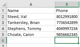
Let assume that you wanted a list with each element in a column—first name, last name, and a phone number someone can use to make calls. But instead, what you got is a last name and a first name jammed into the same column while only the numbers of a phone number appear down the next column. This can be very visually challenging to use for calls.

• Move your cursor over to C2 and type in the name how you want it to appear.
• Press Enter.
• Go to the Data ribbon element and select Flash Fill.

Now, you will see that it populates the column with the exact information you want. While you can do some complex text functions to parse the information, you don’t need to do that anymore.

• Make sure you have clean columns to the right of the columns you’re parsing.
• In the clean column, type the data you want from the left columns into the first cell.

As you start to type the same solution in the second cell down the column, Excel will pop up an Auto Fill box showing the rest of the solutions for your data.

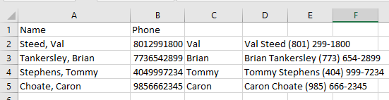
• Hit Enter and it will populate your data down the range.

If the Auto Fill box does not appear type in the first solution, hit CTRL-E for Flash Fill or click to the Data Tab and Select Flash Fill. Remember, this only works on clean columns to the right of the data you are parsing.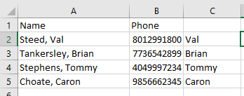 

You can choose what you would like to have as a result. The results are NOT formulas but different arrangements of text. I’ve cut right to the desired list by typing first name, last name, and the phone number the way I want it to appear in D3 and then clicking Flash Fill again. Flash Fill will occasionally bring up the Auto-Complete box if you go down to the second cell in the range and start to typing, but I prefer using the command in the Ribbon or the hot-key CTRL-E.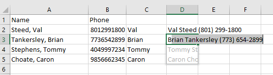





With Flash Fill, you can parse, combine, or add text to your solution. Notice that I added the spaces, parenthesis, and dash.

To see this work at a secondary level, let’s look at a QuickBooks Trial Balance report sent to Excel. Note that the account number, sub account number, and description are all in the same column.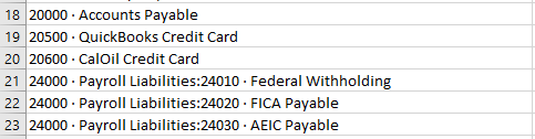 



You’ll notice that we’re headed for a problem. QuickBooks puts the account and sub-account descriptions and account numbers in column A. So, we need to do one more step compared to the first example above.

Flash Fill the account number like you did above and you should end up with the cursor stopping on the first cell with a sub-account.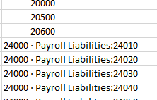 

This is called an ambiguous cell. Excel does not have enough information to solve this secondary level of parse, yet.

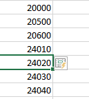
• Type in the proper sub-account number and note that Excel will apply the secondary rule you just taught it to the rest of the data.
  
  
  
  
• Once you have the correct account number, simply Flash Fill the description column and Excel will pick off the appropriate description to match the sub-account as well.
  

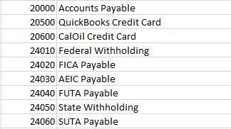
• While this tool will not solve everything, it will take care of a very large percentage of accounting data cleanup issues.

  QuickBooks is notorious for sending over odd formats for reports, so keep an eye out for Text formats on cells. You want either numeric formats for numbers or General for text. I recommend avoiding the actual Text format because it tends to cause formatting issues with QuickBooks data.  

  If you do this right it shouldn’t take you long to split the data into the proper account and description which then allows you to match that up to the amounts.

  Tip #2 - Display of Zeros and Precision as Displayed

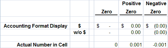
  One of the confounding problems of using any of the financial number formats (Accounting, Currency, and Number) is the display of zeros, which is the third part of any number format code. However, the format code only applies when the value in a cell is equal to zero, not when the value in a cell appears to be zero—such as when a small value rounds off to zero automatically for display. This is especially problematic when using the accounting format because cells can be displayed as zeros, positive zeros, or negative zeros as shown below.
  
  

  Some practitioners have become so frustrated with this problem that they enter hard-coded zeros over formulas when this occurs so that zeros display consistently throughout their reports. This process of overwriting formulas can potentially corrupt your worksheet so that it does not recalculate properly in the future.

  The best solution for all rounding issues is to use Precision as Displayed.

  Precision as Displayed enables global rounding in the affected workbook. When global rounding is enabled, all values are rounded to their cell formats. In other words, the values 0.001 or -0.001 (or smaller)—displayed with two decimals—would automatically be rounded to a cell value of zero.

  Enable Global Rounding in a workbook by clicking:

• “File”
• “Options”
• “Advanced”
• “Set precision as displayed” (near the bottom under the section “When calculating this workbook”)
• “OK”

• Selecting Precision as Displayed will cause Excel to display the warning shown below. 
  

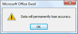
  This does NOT affect any formula. This message is for raw data and only if you have selected fewer decimal places than your raw data. In that case it will round and truncate the raw data. Give this a try and I think you’ll find this old trick to be a go-to tactic this tax season.

  As far as Doug’s question is concerned. We’re not dead yet, so our spreadsheets will live on. Happy computing and all the best this tax season.